Forecasting stock returns can be tempting, it may sound like a good idea but it’s challenging to do accurately and consistently. It’s often best left to well-equipped institutions.

However, it is much easier to predict stock price volatility with a time-series model, for example, the GARCH model. That’s exactly what we are focusing on in this article today. We are going to find the best GARCH model to fit in terms of Autoregressive and Moving Average orders. Then we are going to fit this model and predict in a rolling window the variance of a stock for 1 step ahead, in our case that would be 1 day ahead. After we have all the predictions made, we would be able to compare them to the variance itself and try to form a tradable signal. Let’s get into it!

The development of a volatility model for the stock-returns series is done in four steps:

1. Construct an ARMA model for the financial time series using the serial correlation indicated by the ACF and PACF.
2. Examine the residuals of the model for ARCH/GARCH effects by utilizing the ACF and PACF for the series of squared residuals.
3. If there are significant serial correlation effects, define a volatility model and jointly estimate the mean and volatility equations.
4. Check the fitted model carefully and refine it if necessary.

Project Key Features

• Download daily prices for the last 10 years for the NVDA stock.
• Calculate log returns and plot the autocorrelation and partial-autocorrelation graphs for log returns, then do the same for daily volatility.
• Fit 16 different models of combinations between autoregressive order and moving average order of 1–4, to find the best model, the one minimizing BIC.
• Build a function to fit this best model and predict the next day’s variance. Apply this function on a rolling basis.
• Visualize actual variance and predicted variance, and fix the predictions by applying a Kalman filter noise reduction.
• Calculate prediction premium and form a strategy to invest for 5 days after the signal.

Let’s Get Started

1. Download daily prices for the NVDA stock for a little bit more than 11 years.

import matplotlib.pyplot as plt
import yfinance as yf
import pandas as pd
import numpy as np

stock_df = yf.download(tickers='NVDA', start='2012-01-01', end='2023-01-29')

stock_df

2. Calculate log returns and daily volatility and plot a correlogram for both series.

nvda_log_ret = np.log(stock_df['Adj Close']).diff().dropna()

nvda_daily_vol = (nvda_log_ret-nvda_log_ret.mean())**2

plot_correlogram(x=nvda_log_ret,
                 lags=120,
                 title='NVDA Daily Log Returns')

plot_correlogram(x=nvda_daily_vol,
                 lags=120,
                 title='NVDA Daily Volatility')

From those two plots, we can conclude that there is not enough valuable information into the lags of the log returns to build a reliable model, however, when we look at the daily volatility it looks much better with substantial information and autocorrelation in the lags up to and after 20.

3. Fit 16 different models to find the best model based on 10-year rolling training window.

Here the goal is to fit models with the different orders of Autoregression and Moving Averages, in an attempt to find the model which minimizes the RMSE and BIC. Then after we have found these model orders we can potentially use them to fit and predict in a rolling window.

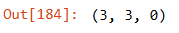
Our brute-force approach yields the conclusion that the best-performing model would be the one with AR order of 3 and MA order of 3.

4. Define a function to predict the next day’s variance using a rolling window, as well calculate the stock variance using the same rolling window.

data = nvda_log_ret.to_frame('nvda_log_ret')

data = data['2020':]

data['variance'] = data['nvda_log_ret'].rolling(70).var()

data['predictions'] = data['nvda_log_ret'].rolling(70).apply(lambda x: predict_volatility(x))

data

5. Plot the predicted variance and the actual rolling variance.

data[['variance', 'predictions']].plot(figsize=(16,4))

plt.title('Compare The Rolling Variance and The Predictions')

plt.show()

It’s looking somewhat good, but the predictions are really messy. What we can do here is just apply a Kalman filter on the predicted values to denoise them.

6. Fix the predictions with a Kalman Filter.

data['fixed_predictions'] = KalmanFilterAverage(data['predictions'])

data[['variance', 'fixed_predictions']].plot(figsize=(16,4))

plt.title('Compare The Rolling Variance and The FIXED Predictions')

plt.show()

Now the predictions look much better and promising 🙂

7. Calculate the predictions premium and form a strategy around.

From this signal, I’ve created a long short strategy with up to a week of holding period.

8. Compare Sharpe ratios of stocks log returns and strategy returns.

print(f"Sharpe Ratio NVDA rets: {round((data['nvda_log_ret'].mean()/data['nvda_log_ret'].std())*(252**.5),2)}")

print(f"Sharpe Ratio strategy rets: {round((data['strategy_return'].mean()/data['strategy_return'].std())*(252**.5),2)}")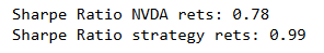

⚠️If you want to get the full code.⚠️

Conclusion

In this article, we explored how to fit a time-series model to successfully predict one day ahead stock variance. Furthermore, we learned how to do that in a rolling window and how to denoise the predictions. In the end, we created a strategy with a holding period of 5 days. If you enjoy such content and are interested in learning much more about algorithmic trading and developing algo trading strategies follow me for more content like this!

I hope this article is helpful! Let me know if you have any questions or if you would like further information on any of the topics covered.

Sources:

Stefan Jansen — Machine Learning for Algorithmic Trading